Many machine studying fashions carry out higher when enter variables are rigorously remodeled or scaled previous to modeling.
It’s handy, and due to this fact widespread, to use the identical knowledge transforms, reminiscent of standardization and normalization, equally to all enter variables. This may obtain good outcomes on many issues. However, higher outcomes could also be achieved by rigorously deciding on which knowledge rework to use to every enter variable previous to modeling.
On this tutorial, you’ll uncover tips on how to apply selective scaling of numerical enter variables.
After finishing this tutorial, you’ll know:
- Tips on how to load and calculate a baseline predictive efficiency for the diabetes classification dataset.
- Tips on how to consider modeling pipelines with knowledge transforms utilized blindly to all numerical enter variables.
- Tips on how to consider modeling pipelines with selective normalization and standardization utilized to subsets of enter variables.
Uncover knowledge cleansing, function choice, knowledge transforms, dimensionality discount and way more in my new guide, with 30 step-by-step tutorials and full Python supply code.
Let’s get began.
Tips on how to Selectively Scale Numerical Enter Variables for Machine Studying
Photograph by Marco Verch, some rights reserved.
Tutorial Overview
This tutorial is split into three components; they’re:
- Diabetes Numerical Dataset
- Non-Selective Scaling of Numerical Inputs
- Normalize All Enter Variables
- Standardize All Enter Variables
- Selective Scaling of Numerical Inputs
- Normalize Solely Non-Gaussian Enter Variables
- Standardize Solely Gaussian-Like Enter Variables
- Selectively Normalize and Standardize Enter Variables
Diabetes Numerical Dataset
As the idea of this tutorial, we are going to use the so-called “diabetes” dataset that has been broadly studied as a machine studying dataset because the 1990s.
The dataset classifies sufferers’ knowledge as both an onset of diabetes inside 5 years or not. There are 768 examples and eight enter variables. It’s a binary classification drawback.
You’ll be able to study extra in regards to the dataset right here:
No must obtain the dataset; we are going to obtain it robotically as a part of the labored examples that comply with.
Wanting on the knowledge, we will see that each one 9 enter variables are numerical.
|
6,148,72,35,Zero,33.6,Zero.627,50,1 1,85,66,29,Zero,26.6,Zero.351,31,Zero eight,183,64,Zero,Zero,23.three,Zero.672,32,1 1,89,66,23,94,28.1,Zero.167,21,Zero Zero,137,40,35,168,43.1,2.288,33,1 … |
We will load this dataset into reminiscence utilizing the Pandas library.
The instance beneath downloads and summarizes the diabetes dataset.
|
# load and summarize the diabetes dataset from pandas import read_csv from pandas.plotting import scatter_matrix from matplotlib import pyplot # Load dataset url = “https://uncooked.githubusercontent.com/jbrownlee/Datasets/grasp/pima-indians-diabetes.csv” dataset = read_csv(url, header=None) # summarize the form of the dataset print(dataset.form) # histograms of the variables dataset.hist() pyplot.present() |
Operating the instance first downloads the dataset and masses it as a DataFrame.
The form of the dataset is printed, confirming the variety of rows, and 9 variables, eight enter, and one goal.
Lastly, a plot is created displaying a histogram for every variable within the dataset.
That is helpful as we will see that some variables have a Gaussian or Gaussian-like distribution (1, 2, 5) and others have an exponential-like distribution (Zero, three, four, 6, 7). This may increasingly counsel the necessity for various numerical knowledge transforms for the various kinds of enter variables.
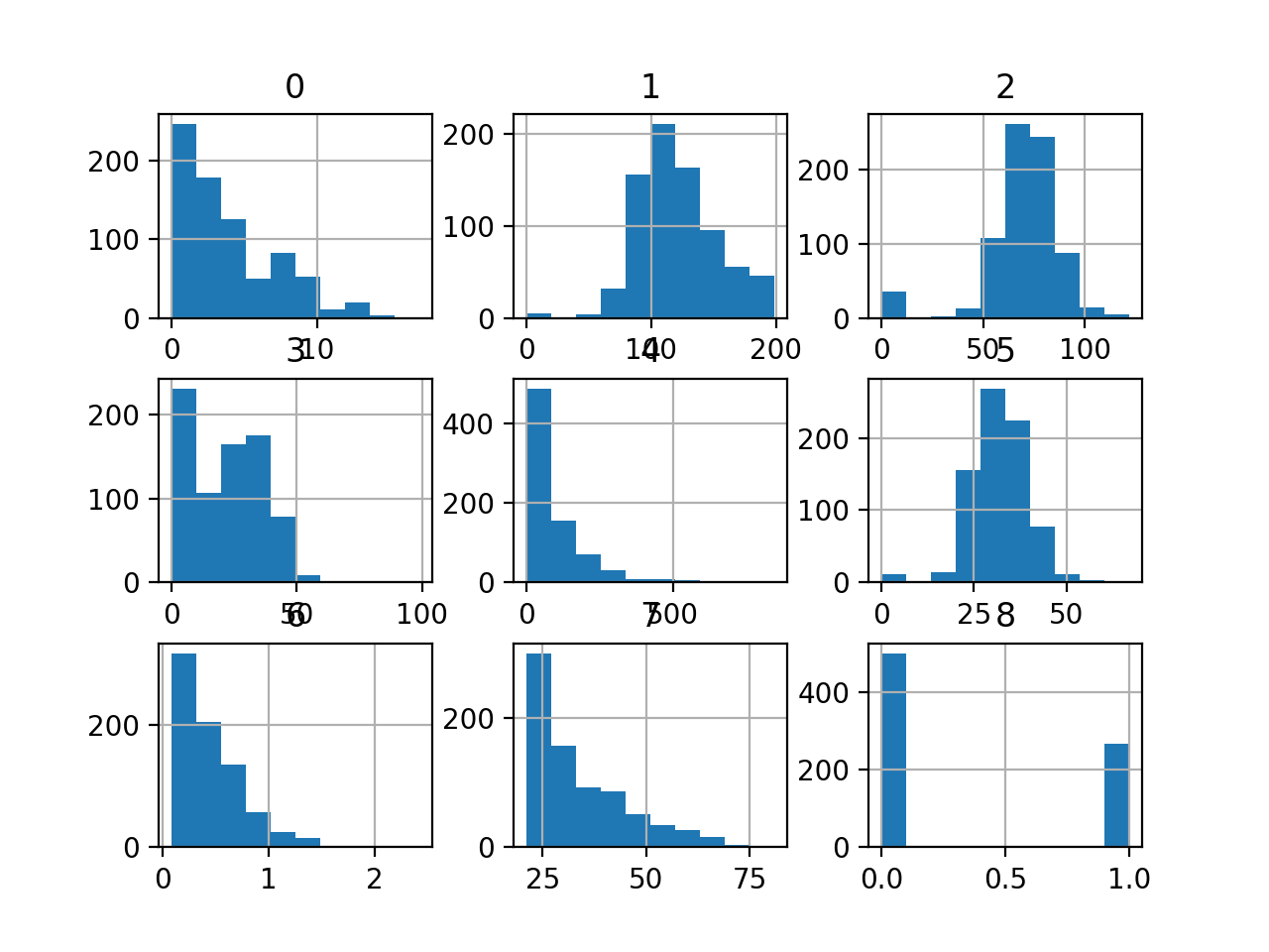
Histogram of Every Variable within the Diabetes Classification Dataset
Now that we’re just a little aware of the dataset, let’s attempt becoming and evaluating a mannequin on the uncooked dataset.
We are going to use a logistic regression mannequin as they’re a strong and efficient linear mannequin for binary classification duties. We are going to consider the mannequin utilizing repeated stratified k-fold cross-validation, a greatest apply, and use 10 folds and three repeats.
The entire instance is listed beneath.
|
1 2 three four 5 6 7 eight 9 10 11 12 13 14 15 16 17 18 19 20 21 22 23 24 25 |
# consider a logistic regression mannequin on the uncooked diabetes dataset from numpy import imply from numpy import std from pandas import read_csv from sklearn.preprocessing import LabelEncoder from sklearn.model_selection import cross_val_score from sklearn.model_selection import RepeatedStratifiedKFold from sklearn.linear_model import LogisticRegression # load dataset url = ‘https://uncooked.githubusercontent.com/jbrownlee/Datasets/grasp/pima-indians-diabetes.csv’ dataframe = read_csv(url, header=None) knowledge = dataframe.values # separate into enter and output parts X, y = knowledge[:, :-1], knowledge[:, -1] # minimally put together dataset X = X.astype(‘float’) y = LabelEncoder().fit_transform(y.astype(‘str’)) # outline the mannequin mannequin = LogisticRegression(solver=‘liblinear’) # outline the analysis process cv = RepeatedStratifiedKFold(n_splits=10, n_repeats=three, random_state=1) # consider the mannequin m_scores = cross_val_score(mannequin, X, y, scoring=‘accuracy’, cv=cv, n_jobs=-1) # summarize the consequence print(‘Accuracy: %.3f (%.3f)’ % (imply(m_scores), std(m_scores))) |
Operating the instance evaluates the mannequin and reviews the imply and normal deviation accuracy for becoming a logistic regression mannequin on the uncooked dataset.
Your particular outcomes might differ given the stochastic nature of the educational algorithm, the stochastic nature of the analysis process, and variations in precision throughout machines and library variations. Attempt working the instance a couple of occasions.
On this case, we will see that the mannequin achieved an accuracy of about 76.eight p.c.
Now that we’ve got established a baseline in efficiency on the dataset, let’s see if we will enhance the efficiency utilizing knowledge scaling.
Need to Get Began With Knowledge Preparation?
Take my free 7-day e-mail crash course now (with pattern code).
Click on to sign-up and likewise get a free PDF E-book model of the course.
Obtain Your FREE Mini-Course
Non-Selective Scaling of Numerical Inputs
Many algorithms favor or require that enter variables are scaled to a constant vary previous to becoming a mannequin.
This consists of the logistic regression mannequin that assumes enter variables have a Gaussian chance distribution. It might additionally present a extra numerically steady mannequin if the enter variables are standardized. However, even when these expectations are violated, the logistic regression can carry out nicely or greatest for a given dataset as could be the case for the diabetes dataset.
Two widespread strategies for scaling numerical enter variables are normalization and standardization.
Normalization scales every enter variable to the vary Zero-1 and could be applied utilizing the MinMaxScaler class in scikit-learn. Standardization scales every enter variable to have a imply of Zero.Zero and an ordinary deviation of 1.Zero and could be applied utilizing the StandardScaler class in scikit-learn.
To study extra about normalization, standardization, and tips on how to use these strategies in scikit-learn, see the tutorial:
A naive method to knowledge scaling applies a single rework to all enter variables, no matter their scale or chance distribution. And that is typically efficient.
Let’s attempt normalizing and standardizing all enter variables instantly and examine the efficiency to the baseline logistic regression mannequin match on the uncooked knowledge.
Normalize All Enter Variables
We will replace the baseline code instance to make use of a modeling pipeline the place step one is to use a scaler and the ultimate step is to suit the mannequin.
This ensures that the scaling operation is match or ready on the coaching set solely after which utilized to the practice and take a look at units throughout the cross-validation course of, avoiding knowledge leakage. Knowledge leakage can lead to an optimistically biased estimate of mannequin efficiency.
This may be achieved utilizing the Pipeline class the place every step within the pipeline is outlined as a tuple with a reputation and the occasion of the rework or mannequin to make use of.
|
... # outline the modeling pipeline scaler = MinMaxScaler() mannequin = LogisticRegression(solver=‘liblinear’) pipeline = Pipeline([(‘s’,scaler),(‘m’,mannequin)]) |
Tying this collectively, the whole instance of evaluating a logistic regression on diabetes dataset with all enter variables normalized is listed beneath.
|
1 2 three four 5 6 7 eight 9 10 11 12 13 14 15 16 17 18 19 20 21 22 23 24 25 26 27 28 29 |
# consider a logistic regression mannequin on the normalized diabetes dataset from numpy import imply from numpy import std from pandas import read_csv from sklearn.preprocessing import LabelEncoder from sklearn.model_selection import cross_val_score from sklearn.model_selection import RepeatedStratifiedKFold from sklearn.pipeline import Pipeline from sklearn.linear_model import LogisticRegression from sklearn.preprocessing import MinMaxScaler # load dataset url = ‘https://uncooked.githubusercontent.com/jbrownlee/Datasets/grasp/pima-indians-diabetes.csv’ dataframe = read_csv(url, header=None) knowledge = dataframe.values # separate into enter and output parts X, y = knowledge[:, :-1], knowledge[:, -1] # minimally put together dataset X = X.astype(‘float’) y = LabelEncoder().fit_transform(y.astype(‘str’)) # outline the modeling pipeline mannequin = LogisticRegression(solver=‘liblinear’) scaler = MinMaxScaler() pipeline = Pipeline([(‘s’,scaler),(‘m’,mannequin)]) # outline the analysis process cv = RepeatedStratifiedKFold(n_splits=10, n_repeats=three, random_state=1) # consider the mannequin m_scores = cross_val_score(pipeline, X, y, scoring=‘accuracy’, cv=cv, n_jobs=-1) # summarize the consequence print(‘Accuracy: %.3f (%.3f)’ % (imply(m_scores), std(m_scores))) |
Operating the instance evaluates the modeling pipeline and reviews the imply and normal deviation accuracy for becoming a logistic regression mannequin on the normalized dataset.
Your particular outcomes might differ given the stochastic nature of the educational algorithm, the stochastic nature of the analysis process, and variations in precision throughout machines and library variations. Attempt working the instance a couple of occasions.
On this case, we will see that the normalization of the enter variables has resulted in a drop within the imply classification accuracy from 76.eight p.c with a mannequin match on the uncooked knowledge to about 76.four p.c for the pipeline with normalization.
Subsequent, let’s attempt standardizing all enter variables.
Standardize All Enter Variables
We will replace the modeling pipeline to make use of standardization as a substitute of normalization for all enter variables previous to becoming and evaluating the logistic regression mannequin.
This is likely to be an acceptable rework for these enter variables with a Gaussian-like distribution, however maybe not the opposite variables.
|
... # outline the modeling pipeline scaler = StandardScaler() mannequin = LogisticRegression(solver=‘liblinear’) pipeline = Pipeline([(‘s’,scaler),(‘m’,mannequin)]) |
Tying this collectively, the whole instance of evaluating a logistic regression mannequin on diabetes dataset with all enter variables standardized is listed beneath.
|
1 2 three four 5 6 7 eight 9 10 11 12 13 14 15 16 17 18 19 20 21 22 23 24 25 26 27 28 29 |
# consider a logistic regression mannequin on the standardized diabetes dataset from numpy import imply from numpy import std from pandas import read_csv from sklearn.preprocessing import LabelEncoder from sklearn.model_selection import cross_val_score from sklearn.model_selection import RepeatedStratifiedKFold from sklearn.pipeline import Pipeline from sklearn.linear_model import LogisticRegression from sklearn.preprocessing import StandardScaler # load dataset url = ‘https://uncooked.githubusercontent.com/jbrownlee/Datasets/grasp/pima-indians-diabetes.csv’ dataframe = read_csv(url, header=None) knowledge = dataframe.values # separate into enter and output parts X, y = knowledge[:, :-1], knowledge[:, -1] # minimally put together dataset X = X.astype(‘float’) y = LabelEncoder().fit_transform(y.astype(‘str’)) # outline the modeling pipeline scaler = StandardScaler() mannequin = LogisticRegression(solver=‘liblinear’) pipeline = Pipeline([(‘s’,scaler),(‘m’,mannequin)]) # outline the analysis process cv = RepeatedStratifiedKFold(n_splits=10, n_repeats=three, random_state=1) # consider the mannequin m_scores = cross_val_score(pipeline, X, y, scoring=‘accuracy’, cv=cv, n_jobs=-1) # summarize the consequence print(‘Accuracy: %.3f (%.3f)’ % (imply(m_scores), std(m_scores))) |
Operating the instance evaluates the modeling pipeline and reviews the imply and normal deviation accuracy for becoming a logistic regression mannequin on the standardized dataset.
Your particular outcomes might differ given the stochastic nature of the educational algorithm, the stochastic nature of the analysis process, and variations in precision throughout machines and library variations. Attempt working the instance a couple of occasions.
On this case, we will see that standardizing all numerical enter variables has resulted in a carry in imply classification accuracy from 76.eight p.c with a mannequin evaluated on the uncooked dataset to about 77.2 p.c for a mannequin evaluated on the dataset with standardized enter variables.
Thus far, we’ve got realized that normalizing all variables doesn’t assist efficiency, however standardizing all enter variables does assist efficiency.
Subsequent, let’s discover if selectively making use of scaling to the enter variables can provide additional enchancment.
Selective Scaling of Numerical Inputs
Knowledge transforms could be utilized selectively to enter variables utilizing the ColumnTransformer class in scikit-learn.
It means that you can specify the rework (or pipeline of transforms) to use and the column indexes to use them to. This may then be used as a part of a modeling pipeline and evaluated utilizing cross-validation.
You’ll be able to study extra about tips on how to use the ColumnTransformer within the tutorial:
We will discover utilizing the ColumnTransformer to selectively apply normalization and standardization to the numerical enter variables of the diabetes dataset to be able to see if we will obtain additional efficiency enhancements.
Normalize Solely Non-Gaussian Enter Variables
First, let’s attempt normalizing simply these enter variables that don’t have a Gaussian-like chance distribution and go away the remainder of the enter variables alone within the uncooked state.
We will outline two teams of enter variables utilizing the column indexes, one for the variables with a Gaussian-like distribution, and one for the enter variables with the exponential-like distribution.
|
... # outline column indexes for the variables with “regular” and “exponential” distributions norm_ix = [1, 2, 5] exp_ix = [Zero, three, four, 6, 7] |
We will then selectively normalize the “exp_ix” group and let the opposite enter variables cross by means of with none knowledge preparation.
|
... # outline the selective transforms t = [(‘e’, MinMaxScaler(), exp_ix)] selective = ColumnTransformer(transformers=t, the rest=‘passthrough’) |
The selective rework can then be used as a part of our modeling pipeline.
|
... # outline the modeling pipeline mannequin = LogisticRegression(solver=‘liblinear’) pipeline = Pipeline([(‘s’,selective),(‘m’,mannequin)]) |
Tying this collectively, the whole instance of evaluating a logistic regression mannequin on knowledge with selective normalization of some enter variables is listed beneath.
|
1 2 three four 5 6 7 eight 9 10 11 12 13 14 15 16 17 18 19 20 21 22 23 24 25 26 27 28 29 30 31 32 33 34 35 |
# consider a logistic regression mannequin on the diabetes dataset with selective normalization from numpy import imply from numpy import std from pandas import read_csv from sklearn.preprocessing import LabelEncoder from sklearn.model_selection import cross_val_score from sklearn.model_selection import RepeatedStratifiedKFold from sklearn.pipeline import Pipeline from sklearn.linear_model import LogisticRegression from sklearn.preprocessing import MinMaxScaler from sklearn.compose import ColumnTransformer # load dataset url = ‘https://uncooked.githubusercontent.com/jbrownlee/Datasets/grasp/pima-indians-diabetes.csv’ dataframe = read_csv(url, header=None) knowledge = dataframe.values # separate into enter and output parts X, y = knowledge[:, :-1], knowledge[:, -1] # minimally put together dataset X = X.astype(‘float’) y = LabelEncoder().fit_transform(y.astype(‘str’)) # outline column indexes for the variables with “regular” and “exponential” distributions norm_ix = [1, 2, 5] exp_ix = [Zero, three, four, 6, 7] # outline the selective transforms t = [(‘e’, MinMaxScaler(), exp_ix)] selective = ColumnTransformer(transformers=t, the rest=‘passthrough’) # outline the modeling pipeline mannequin = LogisticRegression(solver=‘liblinear’) pipeline = Pipeline([(‘s’,selective),(‘m’,mannequin)]) # outline the analysis process cv = RepeatedStratifiedKFold(n_splits=10, n_repeats=three, random_state=1) # consider the mannequin m_scores = cross_val_score(pipeline, X, y, scoring=‘accuracy’, cv=cv, n_jobs=-1) # summarize the consequence print(‘Accuracy: %.3f (%.3f)’ % (imply(m_scores), std(m_scores))) |
Operating the instance evaluates the modeling pipeline and reviews the imply and normal deviation accuracy.
Your particular outcomes might differ given the stochastic nature of the educational algorithm, the stochastic nature of the analysis process, and variations in precision throughout machines and library variations. Attempt working the instance a couple of occasions.
On this case, we will see barely higher efficiency, growing imply accuracy with the baseline mannequin match on the uncooked dataset with 76.eight p.c to about 76.9 with selective normalization of some enter variables.
The outcomes are not so good as standardizing all enter variables although.
Standardize Solely Gaussian-Like Enter Variables
We will repeat the experiment from the earlier part, though on this case, selectively standardize these enter variables which have a Gaussian-like distribution and go away the remaining enter variables untouched.
|
... # outline the selective transforms t = [(‘n’, StandardScaler(), norm_ix)] selective = ColumnTransformer(transformers=t, the rest=‘passthrough’) |
Tying this collectively, the whole instance of evaluating a logistic regression mannequin on knowledge with selective standardizing of some enter variables is listed beneath.
|
1 2 three four 5 6 7 eight 9 10 11 12 13 14 15 16 17 18 19 20 21 22 23 24 25 26 27 28 29 30 31 32 33 34 35 |
# consider a logistic regression mannequin on the diabetes dataset with selective standardization from numpy import imply from numpy import std from pandas import read_csv from sklearn.preprocessing import LabelEncoder from sklearn.model_selection import cross_val_score from sklearn.model_selection import RepeatedStratifiedKFold from sklearn.pipeline import Pipeline from sklearn.linear_model import LogisticRegression from sklearn.preprocessing import StandardScaler from sklearn.compose import ColumnTransformer # load dataset url = ‘https://uncooked.githubusercontent.com/jbrownlee/Datasets/grasp/pima-indians-diabetes.csv’ dataframe = read_csv(url, header=None) knowledge = dataframe.values # separate into enter and output parts X, y = knowledge[:, :-1], knowledge[:, -1] # minimally put together dataset X = X.astype(‘float’) y = LabelEncoder().fit_transform(y.astype(‘str’)) # outline column indexes for the variables with “regular” and “exponential” distributions norm_ix = [1, 2, 5] exp_ix = [Zero, three, four, 6, 7] # outline the selective transforms t = [(‘n’, StandardScaler(), norm_ix)] selective = ColumnTransformer(transformers=t, the rest=‘passthrough’) # outline the modeling pipeline mannequin = LogisticRegression(solver=‘liblinear’) pipeline = Pipeline([(‘s’,selective),(‘m’,mannequin)]) # outline the analysis process cv = RepeatedStratifiedKFold(n_splits=10, n_repeats=three, random_state=1) # consider the mannequin m_scores = cross_val_score(pipeline, X, y, scoring=‘accuracy’, cv=cv, n_jobs=-1) # summarize the consequence print(‘Accuracy: %.3f (%.3f)’ % (imply(m_scores), std(m_scores))) |
Operating the instance evaluates the modeling pipeline and reviews the imply and normal deviation accuracy.
Your particular outcomes might differ given the stochastic nature of the educational algorithm, the stochastic nature of the analysis process, and variations in precision throughout machines and library variations. Attempt working the instance a couple of occasions.
On this case, we will see that we achieved a carry in efficiency over each the baseline mannequin match on the uncooked dataset with 76.eight p.c and over the standardization of all enter variables that achieved 77.2 p.c. With selective standardization, we’ve got achieved a imply accuracy of about 77.three p.c, a modest however measurable bump.
Selectively Normalize and Standardize Enter Variables
The outcomes to this point increase the query as as to whether we will get an additional carry by combining the usage of selective normalization and standardization on the dataset on the identical time.
This may be achieved by defining each transforms and their respective column indexes for the ColumnTransformer class, with no remaining variables being handed by means of.
|
... # outline the selective transforms t = [(‘e’, MinMaxScaler(), exp_ix), (‘n’, StandardScaler(), norm_ix)] selective = ColumnTransformer(transformers=t) |
Tying this collectively, the whole instance of evaluating a logistic regression mannequin on knowledge with selective normalization and standardization of the enter variables is listed beneath.
|
1 2 three four 5 6 7 eight 9 10 11 12 13 14 15 16 17 18 19 20 21 22 23 24 25 26 27 28 29 30 31 32 33 34 35 36 |
# consider a logistic regression mannequin on the diabetes dataset with selective scaling from numpy import imply from numpy import std from pandas import read_csv from sklearn.preprocessing import LabelEncoder from sklearn.model_selection import cross_val_score from sklearn.model_selection import RepeatedStratifiedKFold from sklearn.pipeline import Pipeline from sklearn.linear_model import LogisticRegression from sklearn.preprocessing import MinMaxScaler from sklearn.preprocessing import StandardScaler from sklearn.compose import ColumnTransformer # load dataset url = ‘https://uncooked.githubusercontent.com/jbrownlee/Datasets/grasp/pima-indians-diabetes.csv’ dataframe = read_csv(url, header=None) knowledge = dataframe.values # separate into enter and output parts X, y = knowledge[:, :-1], knowledge[:, -1] # minimally put together dataset X = X.astype(‘float’) y = LabelEncoder().fit_transform(y.astype(‘str’)) # outline column indexes for the variables with “regular” and “exponential” distributions norm_ix = [1, 2, 5] exp_ix = [Zero, three, four, 6, 7] # outline the selective transforms t = [(‘e’, MinMaxScaler(), exp_ix), (‘n’, StandardScaler(), norm_ix)] selective = ColumnTransformer(transformers=t) # outline the modeling pipeline mannequin = LogisticRegression(solver=‘liblinear’) pipeline = Pipeline([(‘s’,selective),(‘m’,mannequin)]) # outline the analysis process cv = RepeatedStratifiedKFold(n_splits=10, n_repeats=three, random_state=1) # consider the mannequin m_scores = cross_val_score(pipeline, X, y, scoring=‘accuracy’, cv=cv, n_jobs=-1) # summarize the consequence print(‘Accuracy: %.3f (%.3f)’ % (imply(m_scores), std(m_scores))) |
Operating the instance evaluates the modeling pipeline and reviews the imply and normal deviation accuracy.
Your particular outcomes might differ given the stochastic nature of the educational algorithm, the stochastic nature of the analysis process, and variations in precision throughout machines and library variations. Attempt working the instance a couple of occasions.

On this case, curiously, we will see that we’ve got achieved the identical efficiency as standardizing all enter variables with 77.2 p.c.
Additional, the outcomes counsel that the chosen mannequin performs higher when the non-Gaussian like variables are left as-is than being standardized or normalized.
I’d not have guessed at this discovering, which highlights the significance of cautious experimentation.
Are you able to do higher?
Attempt different transforms or mixtures of transforms and see in the event you can obtain higher outcomes.
Share your findings within the feedback beneath.
Additional Studying
This part offers extra assets on the subject in case you are seeking to go deeper.
Tutorials
APIs
Abstract
On this tutorial, you found tips on how to apply selective scaling of numerical enter variables.
Particularly, you realized:
- Tips on how to load and calculate a baseline predictive efficiency for the diabetes classification dataset.
- Tips on how to consider modeling pipelines with knowledge transforms utilized blindly to all numerical enter variables.
- Tips on how to consider modeling pipelines with selective normalization and standardization utilized to subsets of enter variables.
Do you’ve gotten any questions?
Ask your questions within the feedback beneath and I’ll do my greatest to reply.
Get a Deal with on Fashionable Knowledge Preparation!
Put together Your Machine Studying Knowledge in Minutes
…with just some strains of python code
Uncover how in my new E-book:
Knowledge Preparation for Machine Studying
It offers self-study tutorials with full working code on:
Characteristic Choice, RFE, Knowledge Cleansing, Knowledge Transforms, Scaling, Dimensionality Discount,
and way more…
Convey Fashionable Knowledge Preparation Strategies to
Your Machine Studying Initiatives
See What’s Inside